Recording data to disk: Difference between revisions
mNo edit summary |
|||
| (3 intermediate revisions by the same user not shown) | |||
| Line 62: | Line 62: | ||
*Other data columns: each channel will have as many columns as the number of acquisitions recorded. This means unprocessed bytevalues, digital channels, decoders and analog operators will all have their columns. Eg, the RAW channels show the raw data the way it comes from the ADC inside the smartscope, so without any kind of filtering or compensation applied to them. | *Other data columns: each channel will have as many columns as the number of acquisitions recorded. This means unprocessed bytevalues, digital channels, decoders and analog operators will all have their columns. Eg, the RAW channels show the raw data the way it comes from the ADC inside the smartscope, so without any kind of filtering or compensation applied to them. | ||
The image below shows an example of how a fastly moving signal can be visualized in Excel. See the next section on more information on how to convert the data discussed above into a graph. | The image below shows an example of how a fastly moving signal can be visualized in Excel. See the next section on more information on how to convert the data discussed above into a graph. | ||
<br><br>'''Note:''' Because of USB bandwidth and disk limitations, it is not possible to record all data to disk. Instead, scopes record short chunks of data, called Acquisitions in the text above. In case of the SmartScope these acquisitions contain 2048 samples, and each acquisition is presented as a separate column. It is important to understand that 2 acquisitions are not consecutive to each other: there is data between them which was not recorded. In case you need consecutive data, switch to Rolling mode instead. | |||
<br>[[File:csvNonRolling.png]] | <br>[[File:csvNonRolling.png]] | ||
==Creating the time axis - visualizing the data in Excel== | ==Creating the time axis - visualizing the data in Excel== | ||
Typically, you’ll want to plot the voltages against the time. The file contains a hidden formula which lets you create the time-axes automatically: select field D3, and double-click on its bottom-right corner. This will make Excel fill the entire column with the timestamp of that acquisition! | Typically, you’ll want to plot the voltages against the time. The file contains a hidden formula which lets you create the time-axes automatically: select field D3, and double-click on its bottom-right corner. This will make Excel fill the entire column with the timestamp of that acquisition! | ||
Latest revision as of 19:48, 22 January 2019
The SmartScope can record all acquired data to readable comma separated values (.csv) files which can be opened with eg Excel, or to much more compact .mat file which can be opened using Matlab or Octave.
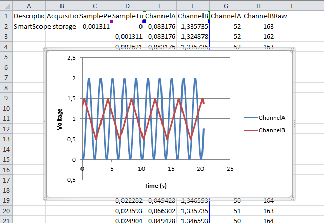
The first secion of this page discusses how to record your acquisitions, while the second section deals with manipulating and visualizing the data recorded to disk.
Selecting the output file type
Start by selecting your output file type at the bottom of the main screen.
Opening and visualizing the contents of these files will be handled further down this document.
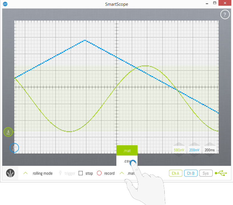
SmartScope recording modes
You can choose between 4 ways of recording your data, each of them explained further on:
- Slow signals, long timespan recording (rolling mode)
- Fast signals, record all data (non-rolling mode)
- Fast signals, record every X seconds (non-rolling mode)
- Full RAM contents (non-rolling mode, single acquisition)
Slow signals, long timespan recording (rolling mode)
In case you want to record slow signals over an extended amount of time, you simply zoom out on the timescale until the SmartScope switches to Rolling mode, and hit the Record button. You should notice the following while recording:
- The Record button is now blinking
- The System measurement box indicates the amount of data stored
- Most GUI elements have been disabled (as otherwise this would invalidate the recording file)
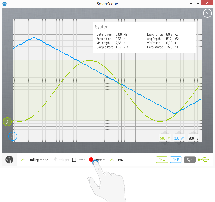
While recording in rolling mode, all channels will be sampled at around 700Hz, and each sample will be stored to file. When you’ve finished recording what you need, simply hit the record button again, and a dialog will show you where the file has been stored.
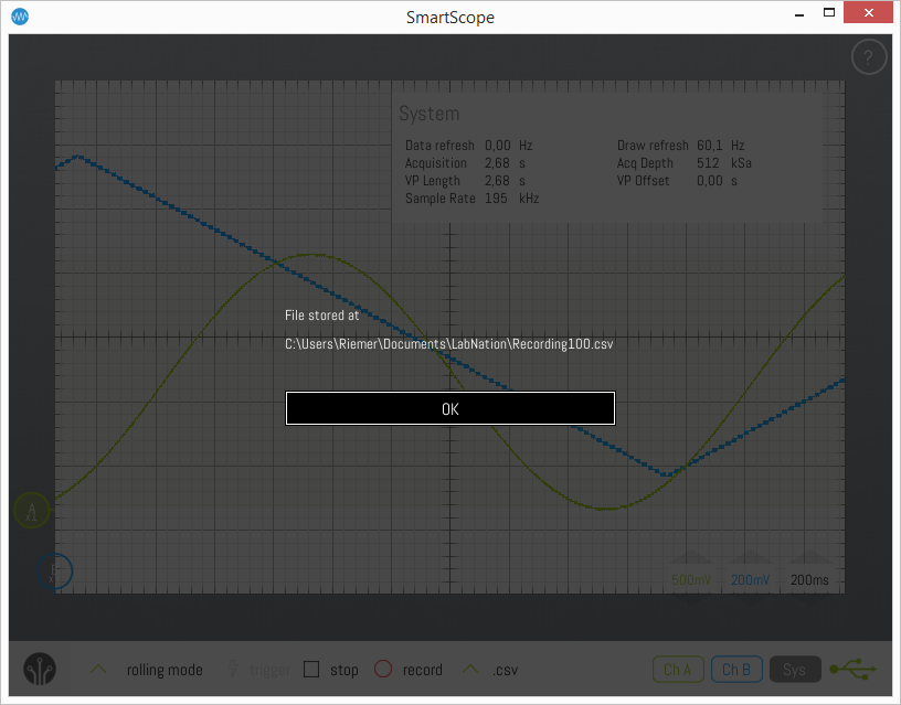
Fast signals, record all data (non-rolling mode)
In case you want to record higher-frequency signals, you’ll typically be out of rolling mode. With sufficiently fast timescale, there can be more than 100 screen updates every second. Every incoming voltage can be saved to disk, simply by hitting the Record button. As long as you’re recording, all incoming data is both stored to disk (hiPriority) and shown on the main graph (lowPriority).
Note: this means the final filesize can grow rapidly! Keep on eye on the ‘Data stored’ entry in the System measurement box. Especially .csv files can grow large, making them very slow to open/handle in Excel.
Fast signals, record every X seconds (non-rolling mode)
The previous scenarios don’t allow you to record for really long timespans (eg hours or days), simply because the amount of data saved to disk would result in huge files. This can be done, but you’ll face trouble when opening them, especially with Excel which is really slow in handling large files.
Instead, the SmartScope allows you to save only 1 recording every X seconds. Or you can also save a burst of Y recordings every X seconds. In order to do this, go to Menu -> System -> Recording, from which you can both set the Interval in seconds (X in the text above), as well as the number of Acquisitions to store in one burst (Y in the text above).
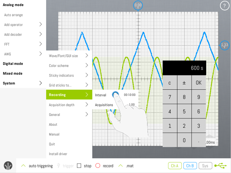
Now when you press the Record button, you’ll see that the ‘Data stored’ property of the Systems measurement box only increases at each interval you specified above. As a result, the file on disk will only contain the bursts at intervals you specify, allowing you to record over very large timespans and still keep the file very small.
Note: this doesn't work in rolling mode. However, while in rolling mode you can always set the the Trigger mode to 'auto trigger'. This gives a visually less appealing result, but allows you to record with a specified interval.
Full RAM contents (single acquisition only)
In all other modes above, all data shown on the screen (and potentially a bit more to the left and right) will be recorded to disk, which typically means 2048 samples for each channel for each acquisition. If you want to store the contents of the full RAM, this is also possible: simply stop the acquisition and wait till the full RAM contents has been downloaded (indicated by the green progress bar in the Panorama). Once this is complete, hit the Record button. You will be presented with the dialog below, asking you if you want to store the current data. When you click OK, the full contents of the RAM will be stored to disk.
Important: You have to wait until the entire contents of the RAM has been transferred (see previous line). When you hit the Record button before this transfer is complete, only the Viewport data (2048 samples) will be written to file.
Note: Excel has a limit of max 1 million rows, so if you’re using csv+Excel make sure you keep the RAM depth to the default setting of 512k.
Working with recorded .csv files
Examining a rolling .csv file data using Excel
Navigate to the recorded file. In case MS Excel is installed on your system, simply double-click the file and its raw contents will be displayed in Excel.
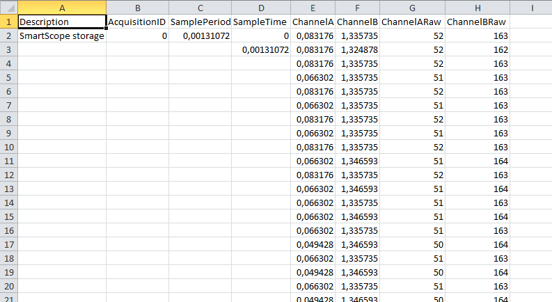
You’ll notice the following columns:
- Description: field containing date and time when the file was created
- AcquisitionID: not used for rolling mode
- SamplePeriod: the amount of seconds between each recorded sample
- SampleTime: useful for creating time axis, see 'Creating the time axis' below
- ChannelA (B): the voltage of ChannelA(B)
- ChannelARaw (B): the unprocessed bytevalue of channel A (B) returned by the hardware
- Channel0-Channel7: in case you've been recording during Mixed mode or Digital mode, the values of the digital channels will be stored to file.
In most cases, you’ll be interested in ChannelA/B columns, as these contain the voltages of both channels. Each row contains a new acquisition, with the time between each acquisition specified in the SamplePeriod column.
Examining a non-rolling .csv file data using Excel
In case your csv file was recorded while not in rolling mode (to record higher-frequency signals), a lot more data will be present in your file. Basically, each waveform displayed while recording will be saved as a column of up to 2048 samples. Simply double-click on the file to open it with Excel.
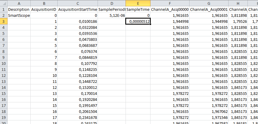
You’ll notice the following columns:
- Description: field containing date and time when the file was created
- AcquisitionID & AcquisitionStartTime: The identier of each acquisition set of 2048 samples, together with the exact timestamp of first sample. This is useful for determining the time between 2 acquisition sets.
- SamplePeriod: the amount of seconds between each recorded sample (between each Excel row)
- SampleTime: useful for creating time axis, see ‘Creating the time axis’ below
From here on, each column represents a full waveform (typically 2048 samples) of the channel specified at the top row:
- ChannelA_Acq00000 -> ChannelA_AcqXYZ: each column represents an acquisition of up to 2048 samples of this channel. These are the voltages measured for the channel written in the top row. The time between each sample (row) is given in the SamplePeriod column (see above). The time between each acquisition set (column) can be derived from the AcquisitionID & AcquisitionStartTime columns (see above)
- Channel[0-7]_Acq00000 -> Channel[0-7]_AcqXYZ: in case you've been recording during Mixed mode or Digital mode, each column here represents an acquisition of up to 2048 digital samples (1 or 0) of all digital channels separately.
- ChannelLA_Acq00000 -> ChannelLA_AcqXYZ: in case you've been recording during Mixed mode or Digital mode, each column here represents an acquisition of up to 2048 byte-value (0 to 255) of all 8 digital inputs combined. This means that these columns are a combination of the Channel[0-7] columns.
- Other data columns: each channel will have as many columns as the number of acquisitions recorded. This means unprocessed bytevalues, digital channels, decoders and analog operators will all have their columns. Eg, the RAW channels show the raw data the way it comes from the ADC inside the smartscope, so without any kind of filtering or compensation applied to them.
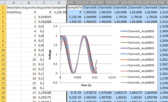
The image below shows an example of how a fastly moving signal can be visualized in Excel. See the next section on more information on how to convert the data discussed above into a graph.
Note: Because of USB bandwidth and disk limitations, it is not possible to record all data to disk. Instead, scopes record short chunks of data, called Acquisitions in the text above. In case of the SmartScope these acquisitions contain 2048 samples, and each acquisition is presented as a separate column. It is important to understand that 2 acquisitions are not consecutive to each other: there is data between them which was not recorded. In case you need consecutive data, switch to Rolling mode instead.
Creating the time axis - visualizing the data in Excel
Typically, you’ll want to plot the voltages against the time. The file contains a hidden formula which lets you create the time-axes automatically: select field D3, and double-click on its bottom-right corner. This will make Excel fill the entire column with the timestamp of that acquisition!

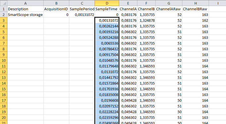
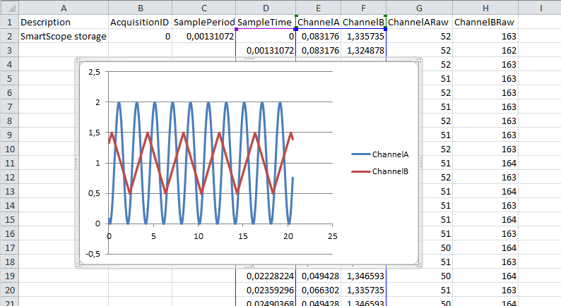
With the time-data and voltage-data present, you can use Excel basics to draw a graph. Simply select the time-data (column D) and voltage-data columns (E and F) by clicking and dragging from D to F on the column names, then go to Insert -> Graph -> Scatter -> Lines.
Working with recorded .mat files
-under construction-